An Example

The Tr-curve

The Tr-curve (Tr stands for thrust required) is a graphical representation of the thrust required by an aircraft to maintain steady and level flight for a range of operating velocities. For an aircraft in steady and level flight (cruise), the thrust required to maintain flight at a particular altitude and velocity is theoritically equal to the drag force experienced by the aircraft. The Tr-curve gives an insight about the aircraft behaviour (stable and unstable flight regions) as it relates to the aircraft velocity. Speaking more about the Tr-curve will be more than the scope of this section, so lets get down to dealing with some aircraft performance problem.

Problem statement

For an aircraft in steady level flight at an altitude of 30,000 ft, plot the Tr-curve for the aircraft between a velocity range of 300 ft/s to 1500 ft/s.

The following are the required aircraft parameters:

weight, W = 73, 000 lb
flight altitude, h = 30, 000 ft
wing span, S = 950 sqr ft
ISA density @ 30,000 ft, po = 0.00089068 slug/cube(ft)
drag polar co.eff, K = 0.08
zero-lift drag, Cd,o = 0.015

Solution

The following are the data required to plot the Tr-curve.

velocity
coefficient of lift, Cl
coeefficient of drag, Cd
thrust required, Tr

So first step, import the neccesary and define the constants

import pandas as pd
import matplotlib.pyplot as plt

from mudu import Force, POUND_FORCE, Length, FOOT, MASS, Mass, Time, SECOND
from mudu.base import _UnitType

SLUG = _UnitType(
    _dimension=MASS,
    _unit_name="slug",
    _unit_symbol="slug",
)

WEIGHT = Force(73_000, POUND_FORCE)
ALTITUDE = Length(30_000, FOOT)
WING_SPAN = 950 * (Length(1, FOOT))**2  # wing_span is in sqr ft
DRAG_POLAR, ZERO_LIFT_DRAG = 0.08, 0.015

# a work around
arb_mass = Mass(1, SLUG)
arb_length = Length(1, FOOT)
arb_volume = arb_length**3
arb_density = arb_mass / arb_volume
DENSITY = 0.00089068 * arb_density

NOTE The code block above has couple of interesting (I hope) manipulations, but lets dig in. First, we created a unit to represent SLUG which is a unit of Mass. Also, when defining the WING_SPAN parameter which is in square feet, we squared the length object which results in a DerivedQuantity and multiplied it with a scalar, it also result is a DerivedQuantity object in square feet. This method is used throughout this example. Similar method is used to define the DENSITY parameter, maybe a bit more elaborate, but quintensentially the same idea.

Next, we continue by defining functions to calculate the coefficient of lift and some lambda to evaluate the coefficient of drag and thrust_required, drag_co_eff and thrust_required respectively.

def lift_co_eff(velocity):

    numerator = 2 * WEIGHT
    denuminator = DENSITY * (velocity**2) * WING_SPAN
    denuminator = Force(denuminator.value, POUND_FORCE) # coercing to pound force

    return numerator / denuminator

drag_co_eff = lambda c_l: ZERO_LIFT_DRAG + (DRAG_POLAR * (c_l**2))
thrust_required = lambda vel, c_d: (0.5) * DENSITY * (vel**2) * WING_SPAN * c_d

then we define a range of velocities for which we are going to calculate the thrust required to maintain the flight at an altitude of 30,000 ft. We also define a list of corresponding coefficients of lift, c_l, coefficients of drag c_d, and thrusts required t_r.

velocity = [(i * Length(1, FOOT)/Time(1, SECOND)) for i in range(300, 1600, 100)]   # v in ft/s
c_l = [round(lift_co_eff(x), 4) for x in velocity]  # dimensionless
c_d = [round(drag_co_eff(c), 4) for c in c_l]   # dimensionless
t_r = [Force(thrust_required(velocity[i], c_d[i]).value, POUND_FORCE) for i in range(len(velocity))]    # in pounds
t_r = [round(x) for x in t_r]

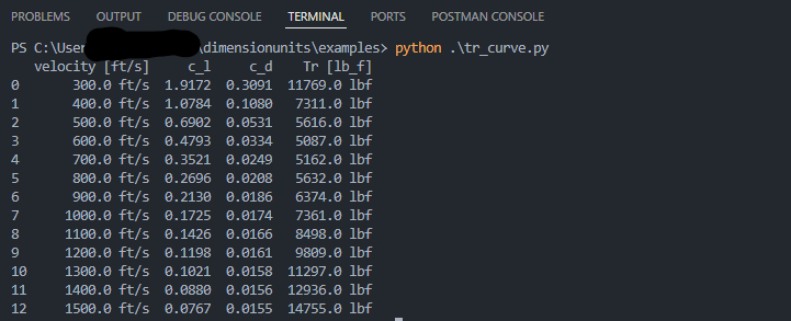
For clarity, we used the pandas DataFrame object to create a table-like structure of our data, printing the data in this format improves data presentation.

df = pd.DataFrame({
    "velocity [ft/s]": velocity,
    "c_l": c_l,
    "c_d": c_d,
    "Tr [lb_f]": t_r
})

print(df)

The result of the above code block looks like this:

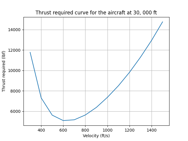
and finally, plotting the graph using matplotlib

vel_values = [x.value for x in velocity]
t_r_values = [y.value for y in t_r]

plt.plot(vel_values, t_r_values, )
plt.title("Thrust required curve for the aircraft")
plt.xlabel("Velocity (ft/s)")
plt.ylabel("Thrust required (lbf)")
plt.grid(True)
plt.show()

The resulting plot looks like this:

In this example, we tried to use as much as object methods as possible to solve the problem at hand with minimal concern for speed, or coding style. This is to emphasise that there are other ways, mostly better ways to solving this problem, exploring those ways is left to the reader.

For more examples, visit the Github repo at https://github.com/techkaduna/mudu.